A familiar example may be useful for understanding the different
fitting options available in the EloOptimized package. We included in
the package a data frame with game results from the 1995-1996 NBA
regular season. We used NBA data because games can’t end in a tie, teams
play all other teams over the course of the season, and there’s a
manageable set of teams for visualization purposes. During the 1995-1996
season, the Chicago Bulls went 72-10 (until recently the best record in
NBA history), had a winning record against all but one team (the Pacers,
against whom they went 2-2), and went on to win the championship.
Therefore we would expect a reasonable ranking method to assign them the
highest rank score by the end of the season. First we’ll use a
traditional Elo ranking approach to assign Elo scores using
eloratingfixed(), and then we’ll show how maximum
likelihood fitting changes ranking.
Traditional Elo scores with default parameter values
First, let’s load the packages we’ll need (we’re using a couple tidyverse packages for post-fitting data manipulation and visualization):
Next, using the nba dataset that’s included with the
EloOptimized package, let’s calculate traditional Elo
scores for each team. Note that you don’t have to supply
pres_data if all individuals (in this case teams) are
present for the entire period of interest.
res = eloratingfixed(agon_data = nba)
#> k = 100
#> prediction accuracy = 0.636
Because we did not specify a k value, the function used the default value of k =100. We find that the prediction accuracy, the proportion of correctly predicted contests, is 0.636.
We can access the data frame of Elo scores using
res$elo, and use ggplot2 to quickly visualize each team’s
trajectory.
head(res$elo)
#>         Date Individual  Elo EloOrdinal EloScaled ExpNumBeaten EloCardinal
#> 1 1995-11-03        ATL  950         15         0     10.26518   0.3801918
#> 2 1995-11-03        BOS  950         16         0     10.26518   0.3801918
#> 3 1995-11-03        CHH  950         17         0     10.26518   0.3801918
#> 4 1995-11-03        CHI 1050          1         1     16.73482   0.6198082
#> 5 1995-11-03        CLE  950         18         0     10.26518   0.3801918
#> 6 1995-11-03        DAL 1050          2         1     16.73482   0.6198082
#>   JenksEloCardinal
#> 1              low
#> 2              low
#> 3              low
#> 4              mid
#> 5              low
#> 6              mid
res$elo %>%
  rename(Team = Individual) %>%
  ggplot(aes(x = Date, y = Elo, color = Team)) +
  geom_line()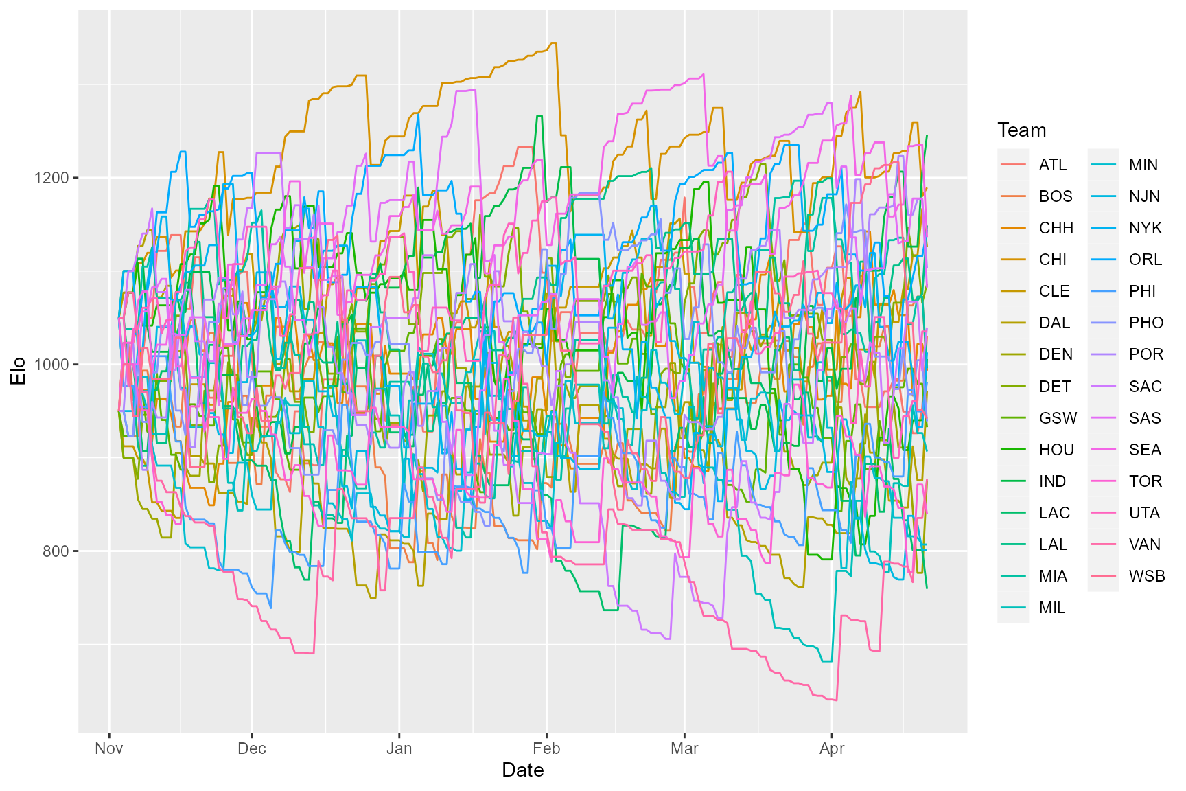
There’s a lot of noise in that plot, but if you look closely you’ll
notice that Chicago doesn’t end the season with the highest Elo score.
There were 29 teams in the NBA in the 95-96 season, so we can check
final Elo scores directly by sorting the the last 29 rows of the Elo
scores data frame (we’re removing a couple columns to make the output
easier to read. See eloratingfixed() documentation for
descriptions of each column):
tail(res$elo, 29) %>% arrange(-Elo) %>% select(-ExpNumBeaten, -JenksEloCardinal)
#>          Date Individual       Elo EloOrdinal  EloScaled EloCardinal
#> 1  1996-04-21        IND 1245.7977          1 1.00000000   0.8921359
#> 2  1996-04-21        CHI 1189.4438          2 0.88412548   0.8285396
#> 3  1996-04-21        LAL 1148.8256          3 0.80060665   0.7710995
#> 4  1996-04-21        ORL 1143.9716          4 0.79062588   0.7636082
#> 5  1996-04-21        SEA 1136.3944          5 0.77504571   0.7516593
#> 6  1996-04-21        CLE 1126.2214          6 0.75412816   0.7351428
#> 7  1996-04-21        POR 1103.2969          7 0.70699086   0.6960572
#> 8  1996-04-21        DET 1085.9874          8 0.67139911   0.6650044
#> 9  1996-04-21        SAS 1082.3680          9 0.66395701   0.6583624
#> 10 1996-04-21        SAC 1039.5035         10 0.57581931   0.5766225
#> 11 1996-04-21        UTA 1035.3141         11 0.56720509   0.5684016
#> 12 1996-04-21        ATL 1030.2344         12 0.55676014   0.5583972
#> 13 1996-04-21        NYK 1012.8371         13 0.52098795   0.5239154
#> 14 1996-04-21        HOU 1005.7356         14 0.50638599   0.5097854
#> 15 1996-04-21        MIA  995.8435         15 0.48604588   0.4900979
#> 16 1996-04-21        CHH  993.8147         16 0.48187438   0.4860634
#> 17 1996-04-21        BOS  992.4673         17 0.47910374   0.4833848
#> 18 1996-04-21        PHI  980.9616         18 0.45544591   0.4605664
#> 19 1996-04-21        DAL  971.1163         19 0.43520196   0.4411554
#> 20 1996-04-21        WSB  941.8334         20 0.37499078   0.3845020
#> 21 1996-04-21        PHO  938.9166         21 0.36899316   0.3789767
#> 22 1996-04-21        GSW  932.6602         22 0.35612873   0.3672130
#> 23 1996-04-21        MIL  906.6344         23 0.30261463   0.3197463
#> 24 1996-04-21        VAN  876.8816         24 0.24143731   0.2689504
#> 25 1996-04-21        DEN  875.6419         25 0.23888825   0.2669245
#> 26 1996-04-21        TOR  839.8903         26 0.16537596   0.2119247
#> 27 1996-04-21        MIN  806.9891         27 0.09772467   0.1675101
#> 28 1996-04-21        NJN  800.9557         28 0.08531886   0.1600331
#> 29 1996-04-21        LAC  759.4621         29 0.00000000   0.1142200
In fact, Indiana ends up with the highest Elo score on the final day. It turns out that they finished the season 8-1 and beat the Bulls in the second to last game of the season. This suggests that the default K parameter of 100 (which determines the degree to which Elo scores change after each contest) is not the best choice. However, it’s not obvious what the K parameter should be set to. Luckily, the EloOptimized package implements a maximum likelihood approach for fitting the K parameter, so you don’t have to make an arbitrary decision.
ML optimized K value
To fit the K parameter, we use eloratingopt():
res2 = eloratingopt(agon_data = nba)
#> k = 20.315
#> prediction accuracy = 0.663
This takes longer than calculating traditional Elo scores because we’re optimizing the K parameter before generating Elo scores. Note that we’re not optimizing K by trying to maximize the prediction accuracy, we’re instead maximizing the likelihood of each contest result according to the sigmoid probability function defined in Foerster, Franz et al., 2016 1. It turns out that the optimized value of K is closer to 20, and this value improves our prediction accuracy to 0.663. Let’s take a look at our results:
res2$elo %>%
  rename(Team = Individual) %>%
  ggplot(aes(x = Date, y = Elo, color = Team)) +
  geom_line()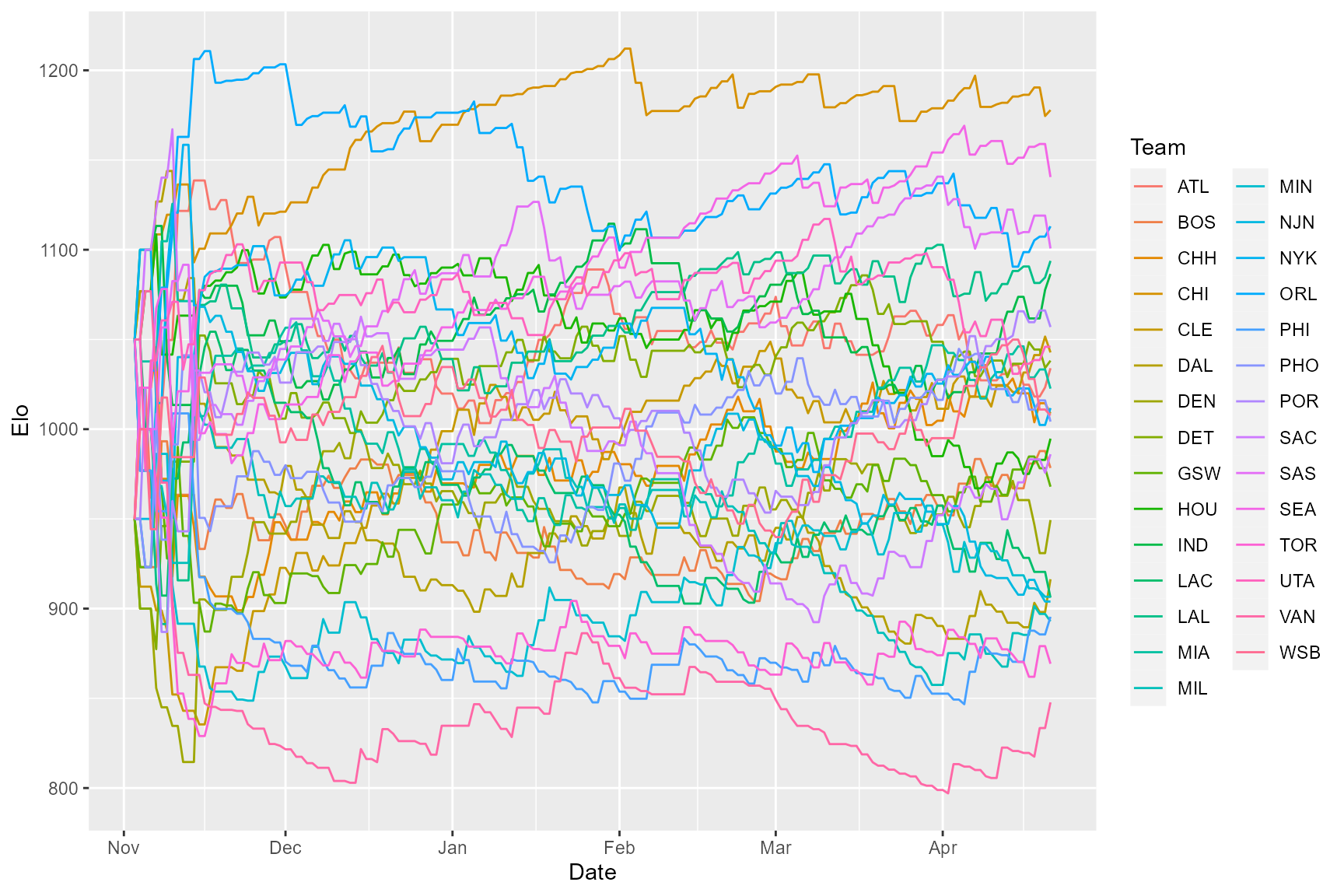
Because eloratingopt() implements a burn-in period of
100 interactions, during which K is fixed at 100, Elo ratings at the
start of the season remain volatile, followed by more stable Elo scores
over the course of the season. It looks like Chicago’s on top this time,
but let’s double check:
tail(res2$elo, 29) %>% arrange(-Elo) %>% select(-ExpNumBeaten, -JenksEloCardinal)
#>          Date Individual       Elo EloOrdinal  EloScaled EloCardinal
#> 1  1996-04-21        CHI 1177.8359          1 1.00000000   0.8386881
#> 2  1996-04-21        SEA 1140.5106          2 0.88692465   0.7832719
#> 3  1996-04-21        ORL 1113.0755          3 0.80381134   0.7361461
#> 4  1996-04-21        SAS 1100.7260          4 0.76639921   0.7132868
#> 5  1996-04-21        LAL 1093.7974          5 0.74540937   0.7000471
#> 6  1996-04-21        IND 1086.4912          6 0.72327570   0.6857814
#> 7  1996-04-21        POR 1056.9233          7 0.63370092   0.6252334
#> 8  1996-04-21        UTA 1045.9352          8 0.60041328   0.6017757
#> 9  1996-04-21        CLE 1042.7688          9 0.59082082   0.5949394
#> 10 1996-04-21        DET 1038.1939         10 0.57696114   0.5850086
#> 11 1996-04-21        ATL 1033.9673         11 0.56415707   0.5757830
#> 12 1996-04-21        MIA 1022.6144         12 0.52976401   0.5508001
#> 13 1996-04-21        NYK 1011.7685         13 0.49690671   0.5267319
#> 14 1996-04-21        CHH 1008.7038         14 0.48762236   0.5199082
#> 15 1996-04-21        WSB 1007.6354         15 0.48438576   0.5175279
#> 16 1996-04-21        PHO 1004.2092         16 0.47400627   0.5098903
#> 17 1996-04-21        HOU  994.7168         17 0.44524936   0.4887185
#> 18 1996-04-21        SAC  986.0321         18 0.41893950   0.4693747
#> 19 1996-04-21        BOS  978.3832         19 0.39576781   0.4523980
#> 20 1996-04-21        GSW  967.9455         20 0.36414713   0.4293813
#> 21 1996-04-21        DEN  949.3502         21 0.30781369   0.3890330
#> 22 1996-04-21        DAL  916.3748         22 0.20791615   0.3206720
#> 23 1996-04-21        MIN  906.6146         23 0.17834829   0.3014633
#> 24 1996-04-21        LAC  906.1413         24 0.17691444   0.3005454
#> 25 1996-04-21        NJN  903.9353         25 0.17023146   0.2962846
#> 26 1996-04-21        PHI  895.4348         26 0.14447960   0.2801379
#> 27 1996-04-21        MIL  892.9171         27 0.13685241   0.2754407
#> 28 1996-04-21        TOR  869.2546         28 0.06516794   0.2333204
#> 29 1996-04-21        VAN  847.7431         29 0.00000000   0.1984100
With K optimized, Chicago ends the season with the highest Elo score. The final Elo scores also end up corresponding more closely to the final standings, although they don’t match exactly. For example, the Utah Jazz finished the season with the fifth best record but the eighth best Elo score, which makes sense given their 5-7 record over their last 12 games. But what about that initial period of volatility corresponding to the burn-in period? Can we do better? The EloOptimized package also allows you to fit individual initial Elo scores (in which case no burn-in period is implemented). Let’s see what happens when we do that with the NBA data.
ML optimized K and initial Elo scores
To fit both the K parameter and initial Elo scores, we use
eloratingopt() with fit_init_elo = TRUE:
res3 = eloratingopt(agon_data = nba, fit_init_elo = TRUE)
#> k = 0
#> prediction accuracy = 0.701
This takes quite a bit longer, because we’re going from optimizing one parameter (K) to optimizing 30 parameters (K plus the 29 initial Elo scores). Surprisingly, the optimized value of K is 0 once you’ve fit initial Elo scores, meaning that Elo scores don’t change at all in response to wins and losses. We might take this to mean that, on average, teams’ competitive ability doesn’t change over the course of the season. Note that fitting initial Elo scores with the included male chimpanzee data results in considerably different patterns, so K = 0 is not an inevitable result of fitting initial Elo scores. Note that this time around the prediction accuracy rises to 0.7. Let’s take a look at our results:
res3$elo %>%
  rename(Team = Individual) %>%
  ggplot(aes(x = Date, y = Elo, color = Team)) +
  geom_line()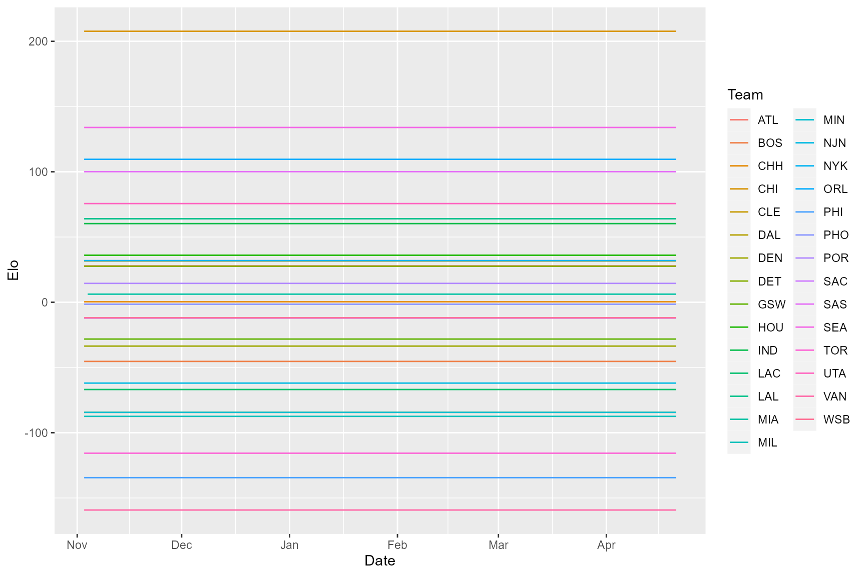
Now Chicago’s dominance is more strongly reflected in their final Elo score relative to others. It’s easier to see this in the EloCardinal scores, which essentially represents the cumulative probability of winning against all other individuals (i.e. teams) scaled by the total number of other individuals/teams.
tail(res3$elo, 29) %>% arrange(-Elo) %>% select(-ExpNumBeaten, -JenksEloCardinal)
#>          Date Individual          Elo EloOrdinal  EloScaled EloCardinal
#> 1  1996-04-21        CHI  207.7177658          1 1.00000000   0.8769118
#> 2  1996-04-21        SEA  133.9553779          2 0.79899641   0.7749567
#> 3  1996-04-21        ORL  109.5561794          3 0.73250823   0.7324324
#> 4  1996-04-21        SAS  100.0777751          4 0.70667944   0.7148051
#> 5  1996-04-21        UTA   75.6299080          5 0.64005864   0.6667434
#> 6  1996-04-21        LAL   63.9886291          6 0.60833598   0.6426847
#> 7  1996-04-21        IND   60.2850436          7 0.59824366   0.6348915
#> 8  1996-04-21        HOU   36.0426311          8 0.53218273   0.5824942
#> 9  1996-04-21        NYK   31.9198718          9 0.52094815   0.5733856
#> 10 1996-04-21        CLE   31.6215718         10 0.52013528   0.5727247
#> 11 1996-04-21        ATL   27.8710139         11 0.50991495   0.5643969
#> 12 1996-04-21        DET   27.5978388         12 0.50917054   0.5637890
#> 13 1996-04-21        POR   14.4577181         13 0.47336352   0.5343736
#> 14 1996-04-21        MIA    6.1987047         14 0.45085759   0.5157586
#> 15 1996-04-21        CHH    0.3442824         15 0.43490420   0.5025331
#> 16 1996-04-21        PHO   -1.5218941         16 0.42981884   0.4983151
#> 17 1996-04-21        WSB  -11.8944890         17 0.40155337   0.4748806
#> 18 1996-04-21        SAC  -12.1603637         18 0.40082886   0.4742806
#> 19 1996-04-21        GSW  -28.2099584         19 0.35709347   0.4382166
#> 20 1996-04-21        DEN  -33.6069809         20 0.34238651   0.4261899
#> 21 1996-04-21        BOS  -45.3500183         21 0.31038656   0.4002799
#> 22 1996-04-21        NJN  -61.9690707         22 0.26509940   0.3644047
#> 23 1996-04-21        LAC  -66.8878710         23 0.25169559   0.3540043
#> 24 1996-04-21        MIN  -84.3953176         24 0.20398754   0.3179502
#> 25 1996-04-21        DAL  -84.3953296         25 0.20398751   0.3179502
#> 26 1996-04-21        MIL  -87.4706128         26 0.19560732   0.3117874
#> 27 1996-04-21        TOR -115.7083976         27 0.11865894   0.2579219
#> 28 1996-04-21        PHI -134.4412811         28 0.06761155   0.2251684
#> 29 1996-04-21        VAN -159.2527265         29 0.00000000   0.1857691
Because each team plays the same number of games, and schedules are fairly balanced, the Elo scores now reflect each team’s overall record. These scores are not useful as dynamic records of team performance, but would be useful for calculating winning probabilities according to the sigmoid equation from Foerster, Franz et al., 2016. And in an animal system where individuals enter and leave the hierarchy through maturation and death, respectively, and where individuals tend to enter towards the bottom of the hierarchy, such a result would reflect a queuing system, as argued in the linked article.
Currently the only option available in the
eloratingopt()function is to use the sigmoid function from the linked paper, but you can use the the pnorm-based method from the EloRating package in theeloratingfixed()function (to make comparison with that package easier).↩︎